LAPOP Visualization Guide
lapop-visualization.RmdIntroduction
This vignette demonstrates how to use the lapop package
to reproduce figures style from the 2023 Pulse of Democracy
report.
Attention: we are only using a subset from the data used in the actual report.
Load Packages
The lapop package brings two datasets already with design effects (weighted).
# Single-country Single-year AmericasBarometer 2023 Brazil
data(bra23)

# AmericasBarometer 2006-2023 Brazil Merge
data(cm23)

# AmericasBarometer 2023 Year Merge
data(ym23)
Survey Design for the Data
The AmericasBarometer use weight1500 for comparative
datasets by time or country, wt weights are only for
country specific datasets (single-country single-year). In the
AmericasBarometer the primary sampling units (ids = upm) and
stratification variable (strata = strata) to account for the survey’s
complex design. Finally, PSUs are nested within strata, properly
reflecting the survey’s hierarchical sampling structure. The
lpr_data() function apply survey design effects.
## Stratified 1 - level Cluster Sampling design (with replacement)
## With (125) clusters.
## Called via srvyr
## Sampling variables:
##   - ids: upm
##   - strata: strata
##   - weights: wt
## Data variables:
##   - ing4 (int), b13 (int), b21 (int), b31 (int), b12 (int), fs2 (fct), idio2
##     (fct), wealth (int), wave (fct), pais (fct), year (fct), upm (int), strata
## (dbl), wt (dbl), pais_lab (chr)## Stratified 1 - level Cluster Sampling design (with replacement)
## With (3943) clusters.
## Called via srvyr
## Sampling variables:
## - ids: upm
## - strata: strata
## - weights: weight1500
## Data variables:
## - ing4 (int), b13 (int), b21 (int), b31 (int), wave (fct), pais (fct), year
## (fct), upm (int), strata (dbl), weight1500 (dbl), pais_lab (chr)## Stratified 1 - level Cluster Sampling design (with replacement)
## With (7856) clusters.
## Called via srvyr
## Sampling variables:
## - ids: upm
## - strata: strata
## - weights: weight1500
## Data variables:
## - b12 (dbl+lbl), b18 (dbl+lbl), wave (dbl+lbl), pais (dbl+lbl), year
## (dbl+lbl), ing4 (dbl+lbl), pn4 (dbl+lbl), vb21n (dbl+lbl), q14f (dbl+lbl),
## edre (dbl+lbl), wealth (dbl), q1tc_r (dbl+lbl), upm (dbl+lbl), strata
## (dbl), weight1500 (dbl), pais_lab (chr)Fonts for 2023 Pulse of Democracy report.
When you load lapop with library(lapop),
the package now auto-registers the bundled LAPOP fonts and enables the
standard plotting setup. You can still call
lapop::lapop_fonts() manually if you want to re-run font
registration in the current session.
lapop::lapop_fonts() # Re-run font registration explicitly if neededFigure 1.1: Time Series
fig1.1_data <- lpr_ts(cm23w, outcome = "ing4", rec = c(5, 7), use_wave = TRUE)

lapop_ts(fig1.1_data,
         ymin = 50,
         ymax = 80,
         main_title = "Support for democracy decline a decade ago and remains comparatively low in Brazil",
         subtitle = "% who support democracy")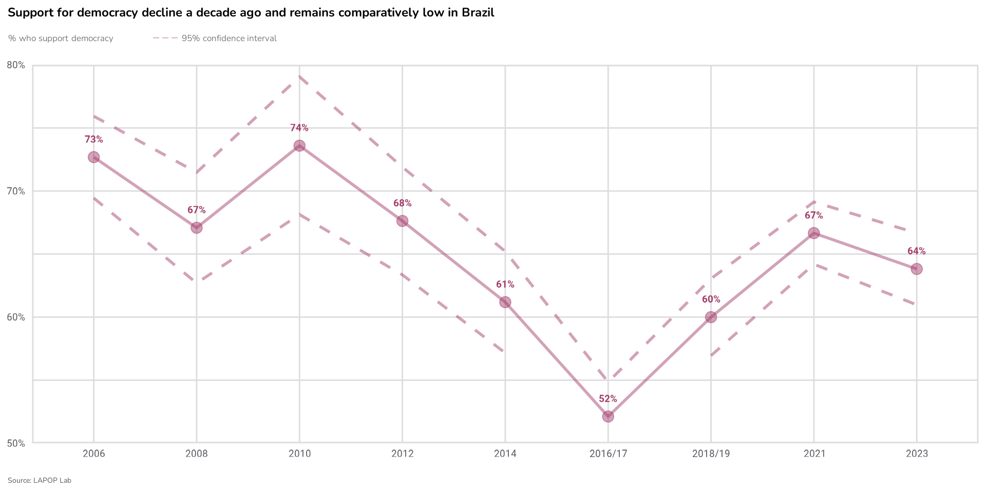
Figure 1.2: Cross-Country Comparison
fig1.2_data <- lpr_cc(ym23w, outcome = "ing4", rec = c(5, 7))

lapop_cc(fig1.2_data,
         main_title = "In many countries, only about one in two adults support democracy",
         subtitle = "% who support democracy")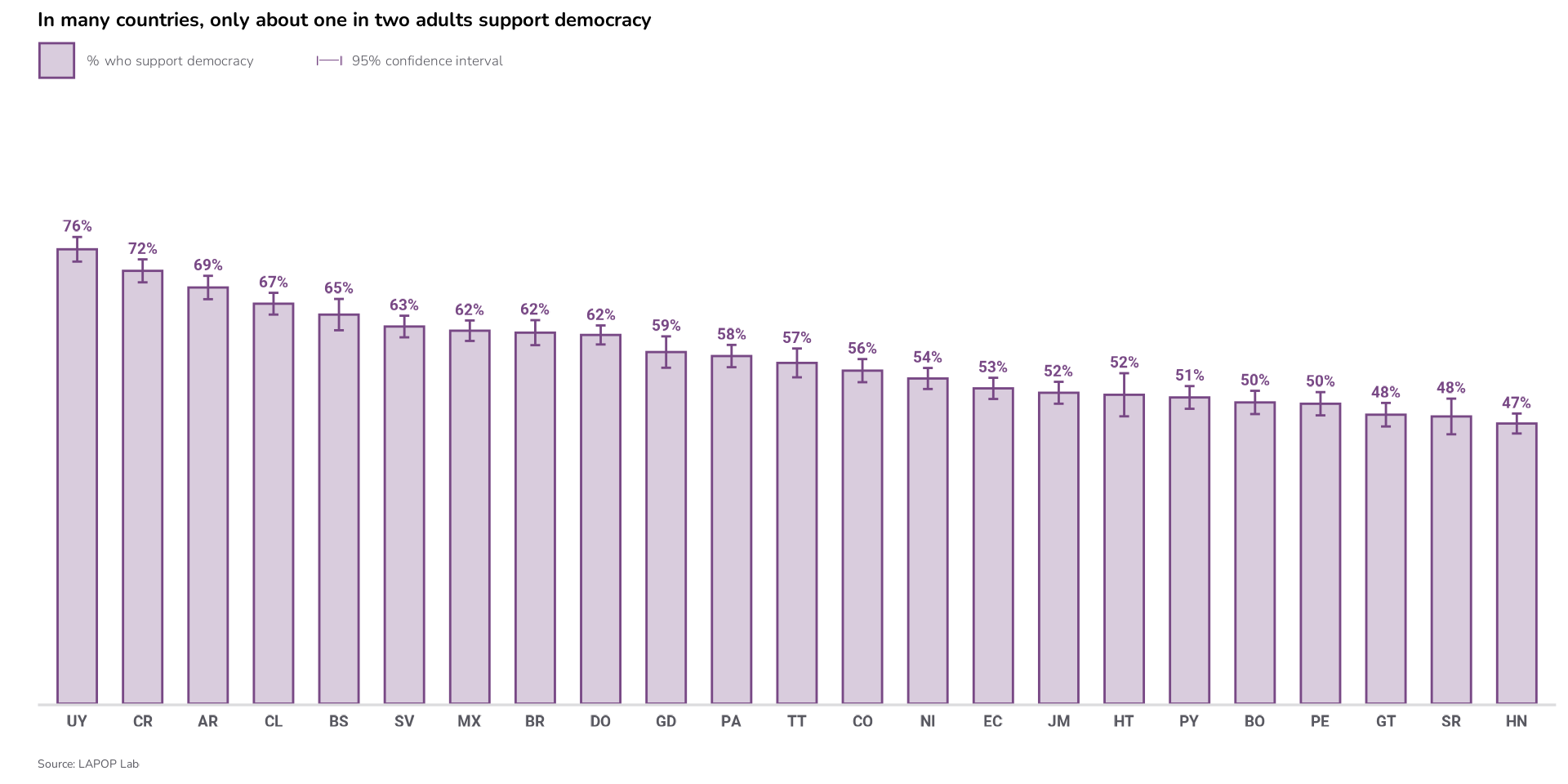
Figure 2.1: Multi-line Over Time
fig2.1_data <- lpr_mline(cm23w,
                         outcome = c("b13", "b21", "b31"),
                         rec = c(5, 7), rec2 = c(5, 7), rec3 = c(5, 7))

# Changing legend for readibility
fig2.1_data$varlabel <- ifelse(fig2.1_data$varlabel == "b13", "National Legislature",
                          ifelse(fig2.1_data$varlabel=="b21", "Political Parties",
                                 "Supreme Court"))

lapop_mline(fig2.1_data,
            main_title = "Trust in executives has declined to a level similar to other \npolitical institutions",
            subtitle = "% who trust...")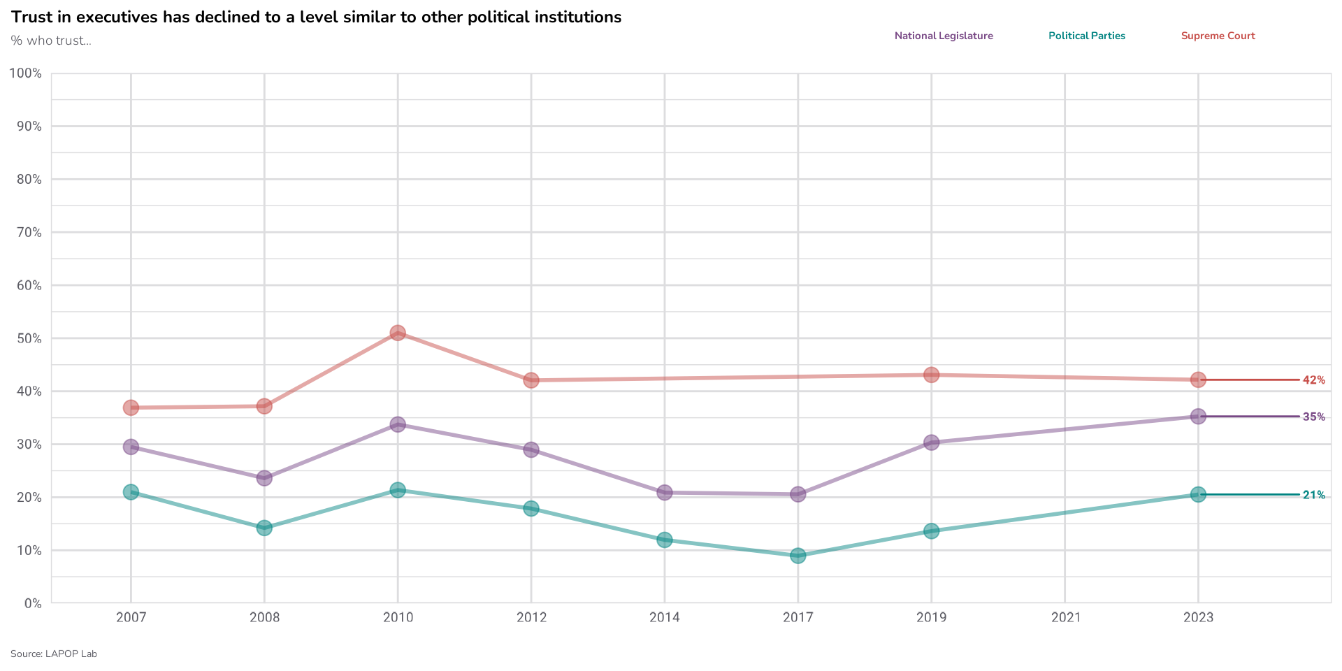
Figure 2.3: CC Multiple Variables
fig2.3_data <- lpr_ccm(ym23w,
                       outcome_vars = c("b12", "b18"),
                       rec1 = c(5, 7),
                       rec2 = c(5, 7))

# Changing legend for readibility
fig2.3_data$var <- ifelse(fig2.3_data$var == "b12", "Armed Forces", "National Police")

lapop_ccm(fig2.3_data,
          main_title = "The public typically reports more trust in the armed forces than the police,\nbut levels vary",
          subtitle = "% who trust...")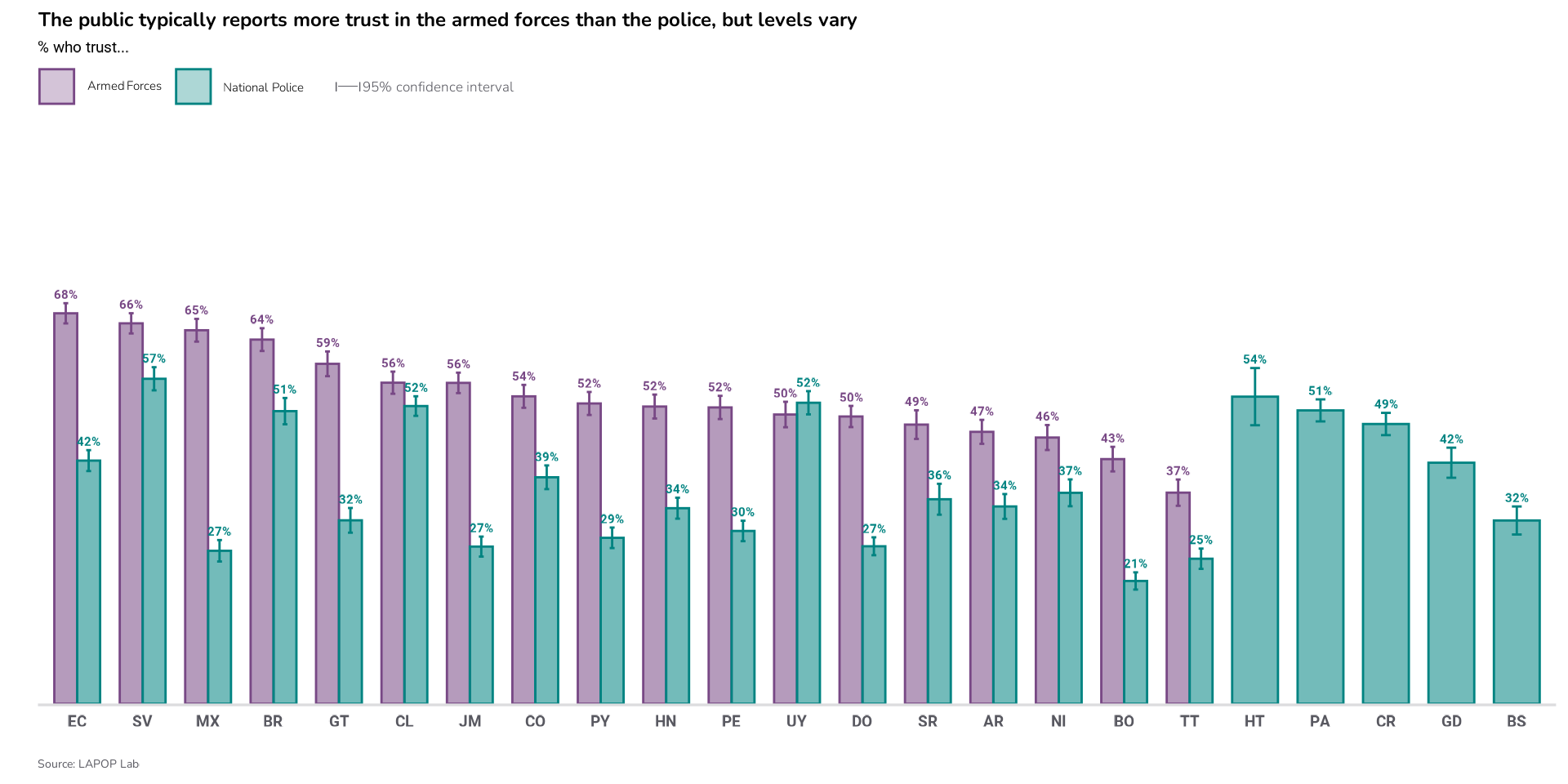
Figure Mover Example: Satisfaction with Democracy
library(dplyr)

ym23w$variables <- ym23w$variables %>%
    mutate(
    edrer = as.numeric(edre),
    gender = as.numeric(q1tc_r)
  ) %>%
  mutate(edrer = case_when(
    edrer <= 2 ~ "None/Primary",
    edrer %in% c(3, 4) ~ "Secondary",
    edrer > 4 ~ "Superior",
    TRUE ~ NA_character_
  ),
  edrer = factor(edrer, levels = c("None/Primary", "Secondary", "Superior")),
  gender = ifelse(q1tc_r == 3, NA, q1tc_r)) %>%
  mutate(gender = case_when(
    gender == 1 ~ "Men",
    gender == 2 ~ "Women",
     TRUE ~ NA_character_
  ))

# Changing legend for readibility
attributes(ym23w$variables$gender)$label <- "Gender"
attributes(ym23w$variables$edrer)$label <- "Education"
attributes(ym23w$variables$wealth)$label <- "Wealth"

fig_mover <- lpr_mover(ym23w,
                       outcome = "pn4",
                       grouping_vars = c("gender", "edrer", "wealth"),
                       rec = c(1, 2))

lapop_mover(fig_mover,
            main_title = "Satisfaction with democracy is significantly lower among women,\nthose with higher educational attainment, and the middle class",
            subtitle = "% who are satisfied with democracy")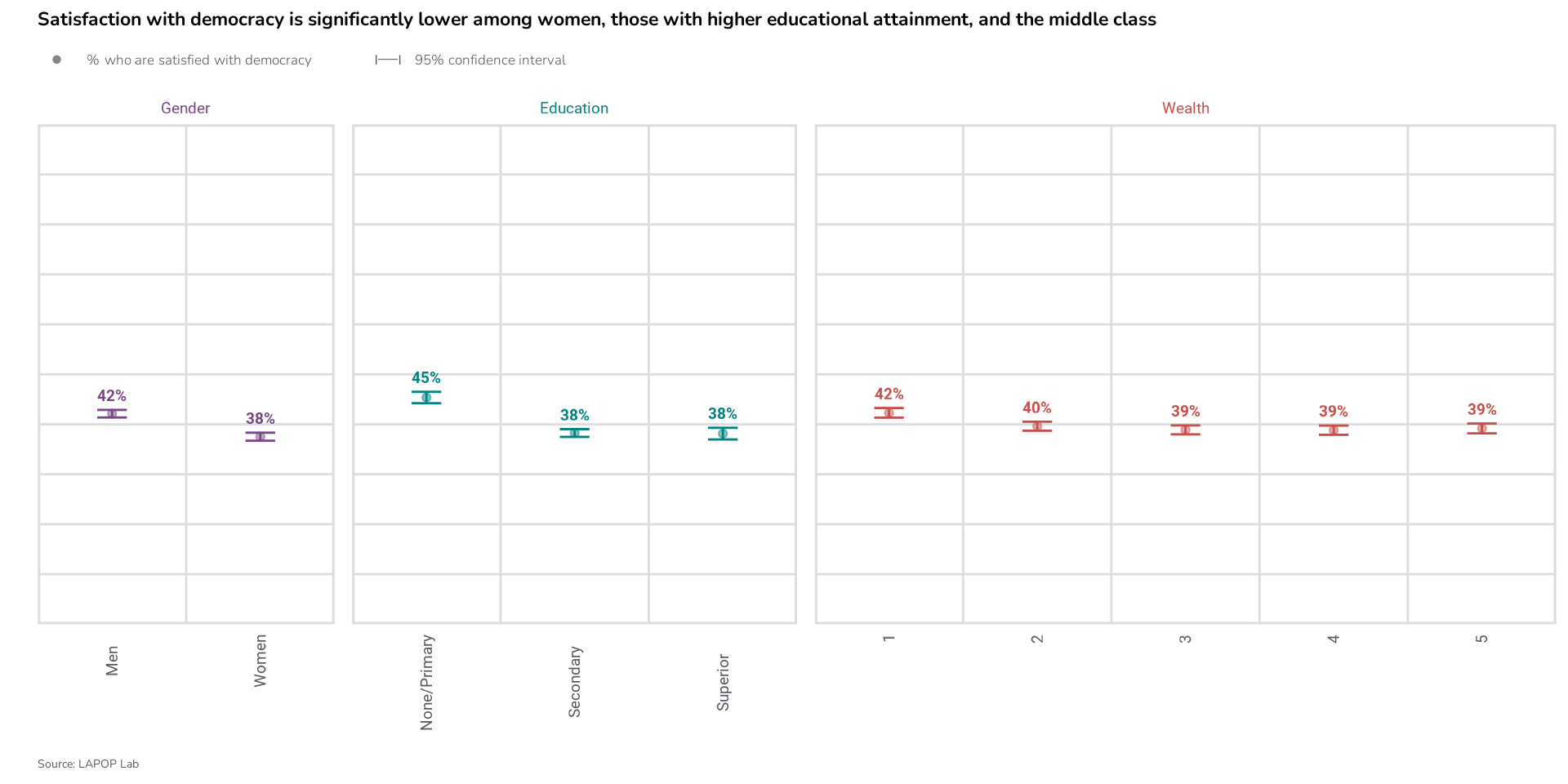
Figure Histogram: Citizens’ Views
spot32_data <- lpr_hist(ym23w, outcome = "vb21n")

# Translating to English
spot32_data$cat <- c("Vote", "Run for\noffice",
                     "Protest",
                     "Participate\nin local orgs.",
                     "Other",
                     "Change is\nimpossible")

lapop_hist(spot32_data,
           main_title = "On average in the LAC region, one in three say voting is the best way \nto influence change",
           subtitle = "How do you believe you can best influence change?")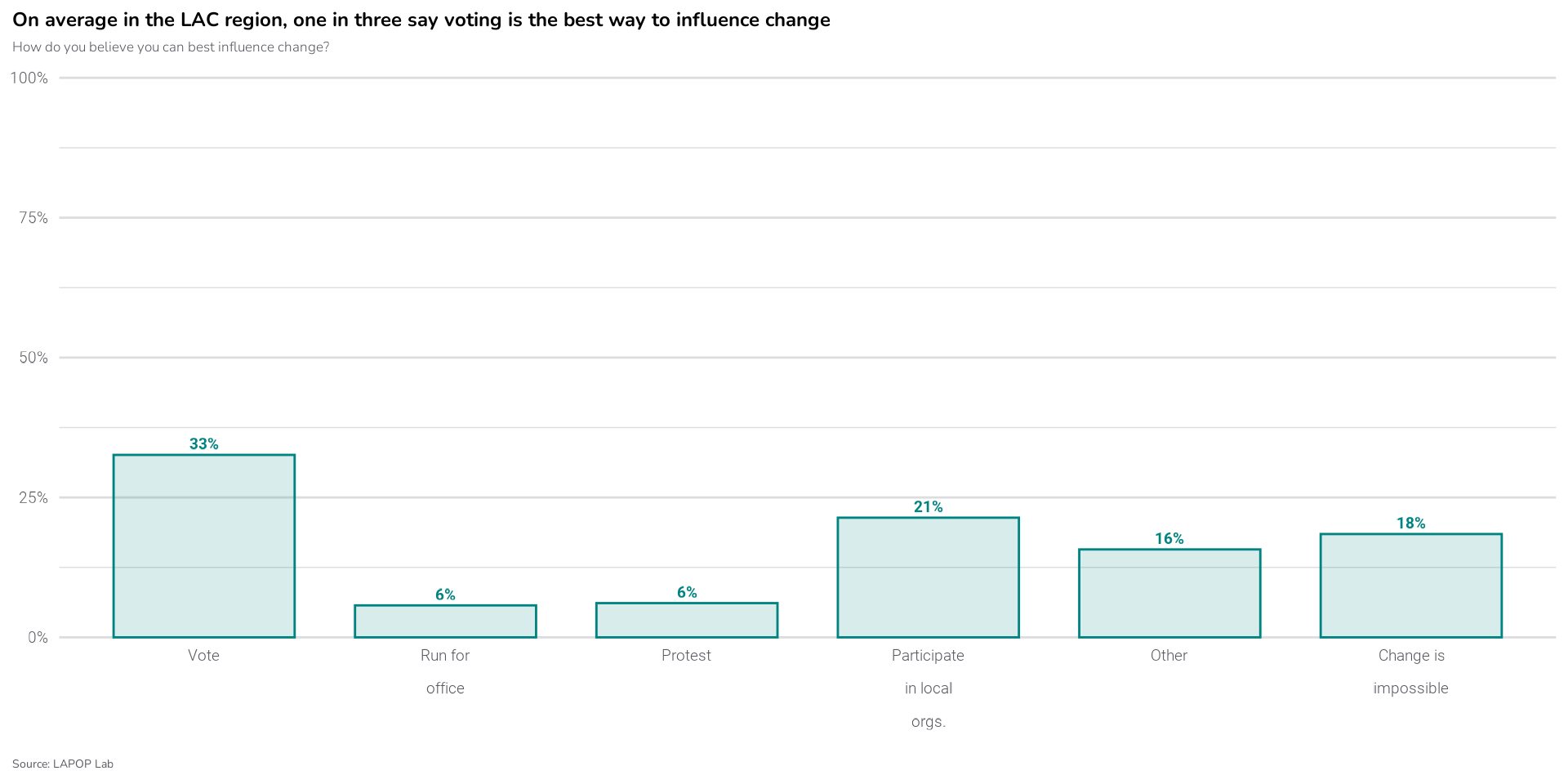
Figure 3.5: Dumbell Plot
fig3.5_data <- lpr_dumb(ym23w,
                        outcome = "q14f",
                        rec = c(1, 1),
                        over = c(2018, 2023),
                        xvar = "pais",
                        ttest = TRUE)

# Select Countries
fig3.5_data <- fig3.5_data[c(1:3,5:6), ]

lapop_dumb(fig3.5_data,
           main_title = "Among those with emigration intentions, the percentage who say they are \nvery likely to emigrate increased in Nicaragua and Guatemala",
           subtitle = "% who say it is very likely they will emigrate",
           source = "LAPOP Lab, AmericasBarometer 2018/19 and 2023")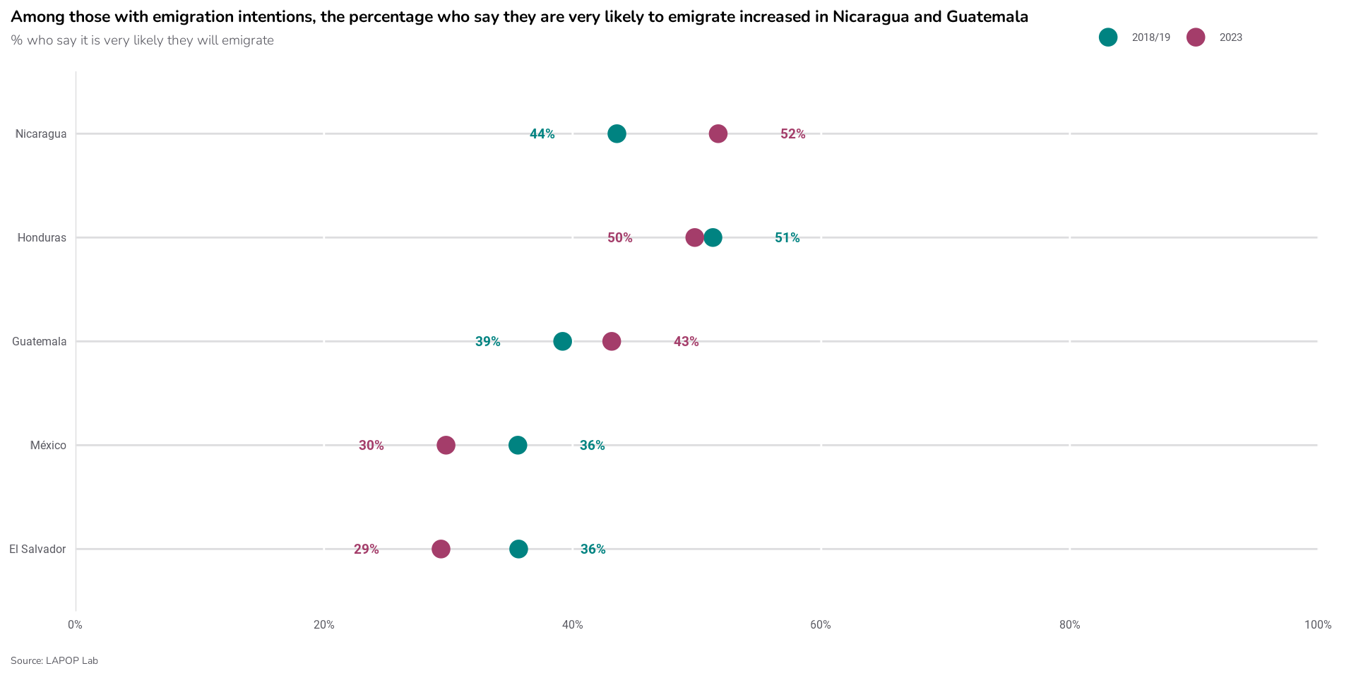
Figure 3.8: Stack Plot by Country
attributes(ym23w$variables$q14f)$label <- "Migration intentions"

fig3.8_data <- lpr_stack(ym23w,
                         outcome = "q14f",
                         xvar = "pais",
                         order = "hi-lo")

lapop_stack(fig3.8_data,
            xvar = "xvar_label",
            source = "LAPOP Lab, AmericasBarometer 2023",
            main_title = "Nicaragua has the highest percentage of individuals with migration intentions,\nwhile Haiti has the lowest")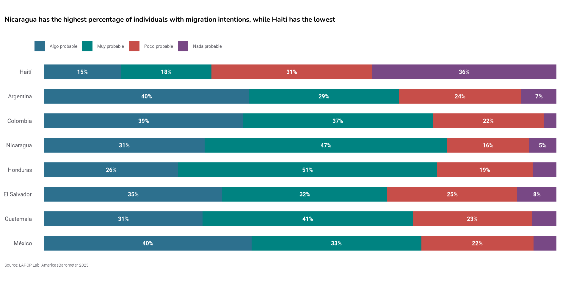
Bonus: Reverse Variables
According to the LAPOP Editorial Guidelines, when variables are measured on a scale, reversing them can enhance clarity and coherence in data representation. For instance, if a survey question aims to measure positive sentiment but higher numeric values indicate negative responses, reversing the variable aligns the coding with the expected direction of responses. This makes it easier for readers to understand the findings.
# For data.frames
cm23$ing4r <- lpr_resc(cm23$ing4, reverse = TRUE, map=TRUE)
##
## 1 2 3 4 5 6 7
## 1 0 0 0 0 0 0 928
## 2 0 0 0 0 0 660 0
## 3 0 0 0 0 1274 0 0
## 4 0 0 0 2112 0 0 0
## 5 0 0 2811 0 0 0 0
## 6 0 2374 0 0 0 0 0
## 7 4952 0 0 0 0 0 0
# For LPR_DATA() objects
cm23w$variables$ing4r <- lpr_resc(cm23w$variables$ing4, reverse = TRUE, map=TRUE)
##
## 1 2 3 4 5 6 7
## 1 0 0 0 0 0 0 928
## 2 0 0 0 0 0 660 0
## 3 0 0 0 0 1274 0 0
## 4 0 0 0 2112 0 0 0
## 5 0 0 2811 0 0 0 0
## 6 0 2374 0 0 0 0 0
## 7 4952 0 0 0 0 0 0End
This vignette is intended as a template and starting point for your own reports and exploratory visualizations using LAPOP data.
By adapting these examples, you can produce consistent, high-quality charts that follow the LAPOP Lab’s editorial guidelines and communicate survey results effectively.
For further guidance:
-
Function documentation: See the package help pages
for detailed arguments and examples (e.g.,
?lpr_cc,?lapop_cc). - Editorial guidelines: Follow LAPOP Lab’s recommendations for plot labeling to ensure clarity and comparability.
- More articles: Check other vignettes and the pkgdown site for additional tutorials and updates.
If you encounter any issues or have suggestions for improvement, please let us know via our GitHub issues page.
Thank you for using the LAPOP R package to help make high-quality, reproducible social science research easier and more accessible!